globe.c

I recently decided to write a parser for NOAA's Global Land One-kilometer Base Elevation (GLOBE) dataset. Compiled in 1999, GLOBE is a coarse resolution dataset, suitable for climate/weather modelling, non-safety-critical navigation aids, and other tasks where a finer-grained model is not necessary. This dataset is a convenient format for projects that need to approximate the geological features of the Earth on a global scale while maintaining a lightweight memory footprint. 1km resolution is higher than the resolution of most weather models, such as the Global Forecast System, which has a 28km horizontal resolution, and it is a good starting point for applications like games and global basemaps.

Size

Weighing in at 1.8GB raw, GLOBE has a simple file format. The dataset is divided into 18 spatial partitions, each representing a 30 arc-second grid of lon/lat centroids. The files each contain a block of 16 bit signed integers (int16_t), making it straightforward to load in any language that can read contiguous arrays from disk. For example, in python, you could do something like:

np.fromfile('./a10g', dtype=np.int16)

...or in node.js:

new Int16Array(fs.readFileSync('./a10g'))

This is a common way to pass assets around in game development, but not so common anywhere else these days. Most modern geospatial file types have complex header schemas, hierarchical structures, and nested format types. GLOBE follows an older model, where the "header" is a detailed PDF specification describing the data, and the data is just... the data. Refreshingly simple!

Partition structure

The file name is used to convey metadata about each file. The first character of the file name represents the spatial partition, followed by a version number. So a11g is the Alaska partition, version 11. NOAA provides the following image to explain this structure:

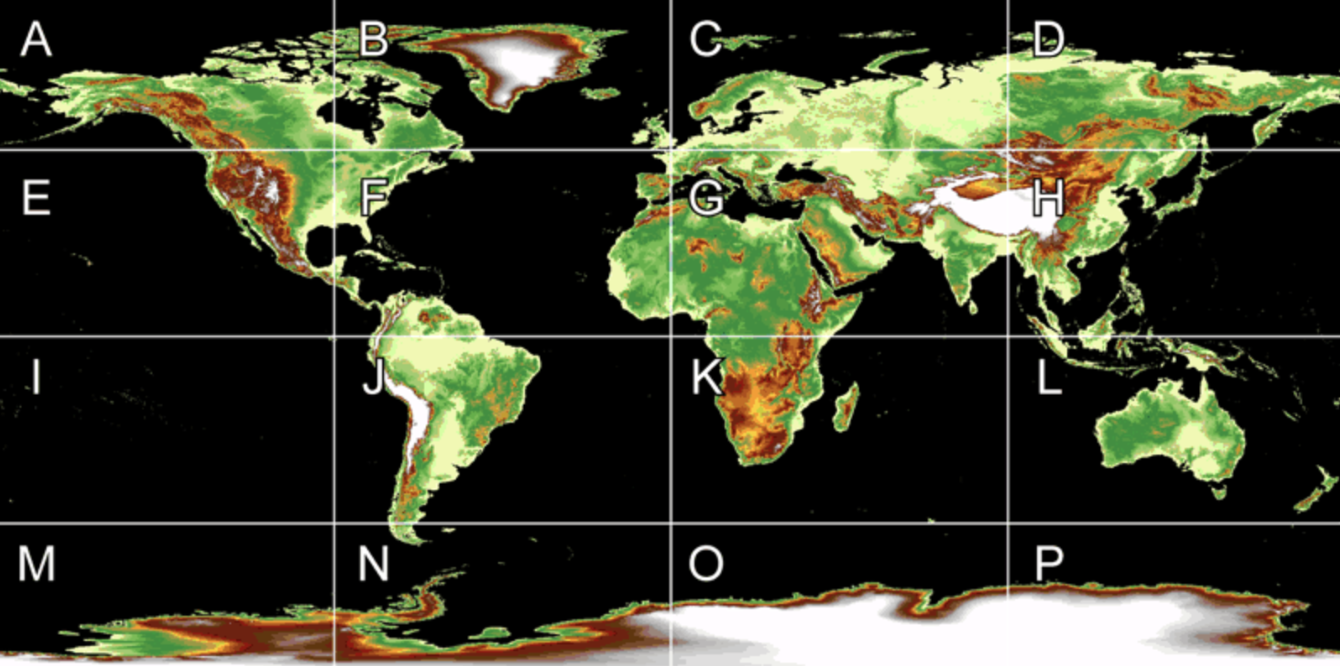
globe.c

globe.c is a parser and toolset for NOAA's Global Land One-kilometer Base Elevation (GLOBE) dataset. It has zero dependencies and is written in C99. It is capable of flattening the raw grids into a single file, making it easier to load and manipulate in memory. While the spatial sharding was a necessary convenience in 1999, today we can easily fit the entire dataset into a single file on disk, and even a single array in memory. This makes it possible to load the entire globe in a single line of code in most programming languages without the need for an API of any kind.

globe merge -o ./globe.bin;
node -e "console.log(new Int16Array(fs.readFileSync('./globe.bin')))"
    Int16Array(1866240000) [
        12, 254, 12, 254, 12, 254, 12, 254, 12, 254, 12, 254,
        12, 254, 12, 254, 12, 254, 12, 254, 12, 254, 12, 254,
        12, 254, 12, 254, 12, 254, 12, 254, 12, 254, 12, 254,
        12, 254, 12, 254, 12, 254, 12, 254, 12, 254, 12, 254,
        12, 254, 12, 254, 12, 254, 12, 254, 12, 254, 12, 254,
        12, 254, 12, 254, 12, 254, 12, 254, 12, 254, 12, 254,
        12, 254, 12, 254, 12, 254, 12, 254, 12, 254, 12, 254,
        12, 254, 12, 254, 12, 254, 12, 254, 12, 254, 12, 254,
        12, 254, 12, 254,
    ... 1866239900 more items
]

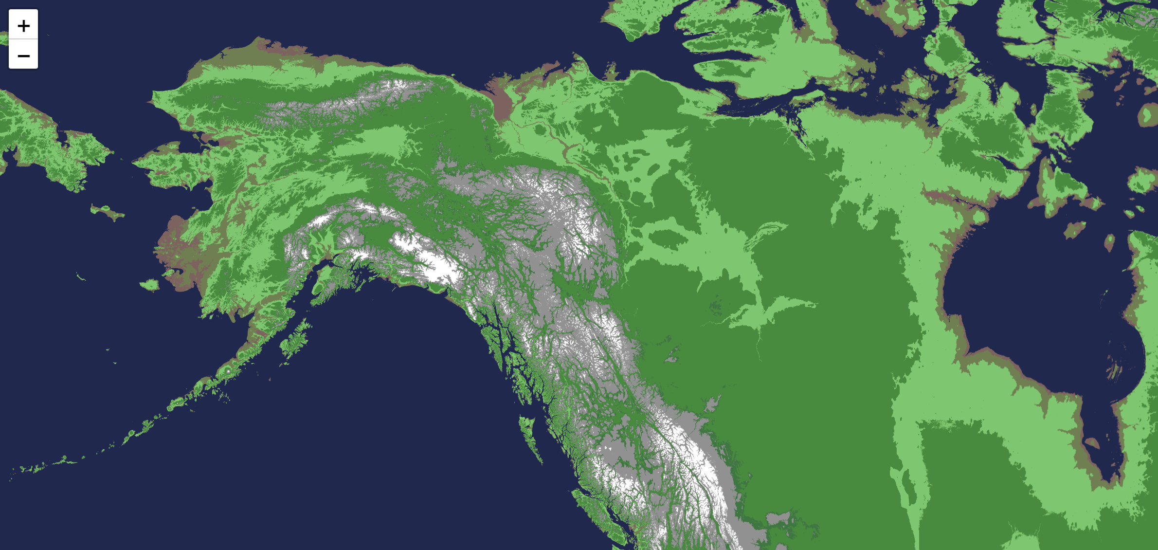
A demo site is available for the project, including a prerendered world map. The provided map is powered by Leaflet, backed by tiles rendered using globe.c, following a standard map tile structure:

globe render -i ./globe.bin -o ./demo/1/0/0.png --minlon=-180 --minlat=0 --maxlon=0 --maxlat=90;
globe render -i ./globe.bin -o ./demo/1/0/1.png --minlon=-180 --minlat=-90 --maxlon=0 --maxlat=0;
[...]

Querying

globe.c can export data as CSV, making it easy to query and analyze. In this example, the csv data is converted to parquet for further analysis using duckdb.

globe table -i ./globe.bin -o globe.csv;
duckdb -c "copy (select * from globe.csv) to 'globe.parquet' \
(FORMAT PARQUET, COMPRESSION ZSTD, ROW_GROUP_SIZE 10_000_000)"

Summary statistics:

select 
    min(elev), 
    quantile_disc(elev, 0.25) as p25, 
    median(elev), 
    avg(elev), 
    quantile_disc(elev, 0.75) 
    as p75, max(elev) 
from './globe.parquet';

# Summary
+-----------+-----+--------------+-------------------+------+-----------+
| min(elev) | p25 | median(elev) |     avg(elev)     | p75  | max(elev) |
+-----------+-----+--------------+-------------------+------+-----------+
| -407      | 219 | 609.0        | 1138.489993141472 | 1950 | 8752      |
+-----------+-----+--------------+-------------------+------+-----------+

Locating the high and low point:

select * from globe.parquet order by elev desc limit 1;

# Himalayas
+-----------+----------+------+
|    lon    |   lat    | elev |
+-----------+----------+------+
| 86.874268 | 28.00589 | 8752 |
+-----------+----------+------+

select * from globe.parquet order by elev asc limit 1;

# Dead Sea
+-----------+-----------+------+
|    lon    |    lat    | elev |
+-----------+-----------+------+
| 35.320187 | 30.997511 | -407 |
+-----------+-----------+------+

The source code is provided under the MIT license.

---

2-27-25